
Everyone who works with data understands that it would be super difficult to read, analyze, and understand without first putting them into a spreadsheet, not to mention the messy and confusing state we would always be in.
Well, it was thanks to Excel first and other tools that come over the years that we even got this wonderful tool available to use, and that has made most jobs out there easier to handle. When talking about jobs, people working in fields where numbers are an inevitable part of it can greatly benefit from this tool.
Why Use Excel Formulas & Functions?
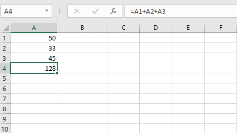
Among the many features of Excel, the formulas and functions are some of the most useful. While function and formulas might sound like they are the same thing, they have a slight difference. Formulas are a set of expressions one can use to calculate the value of the cells. In the example below, the used formula can do the calculation for you; just write down the formula.
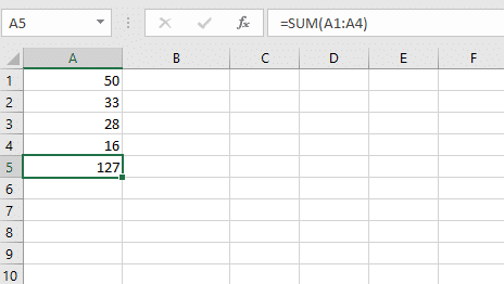
In a way, functions are formulas too. The difference is that they are pre-set, and as such, they are built into Excel. They sort of have the function of a shortcut as by using them you choose a short road to finishing the task, which results in you being able to save time. In the example below, the used SUM function performs the same calculation we did above but with the distinction that it takes less time.
Essential Excel Functions & Formulas to Use
Now that we got it out of the way why one should use Excel formulas, we’re going to focus on the actual formulas that could be convenient for anyone that uses excel on a daily basis regardless of the field they work on (not only the business field).
F4 Key
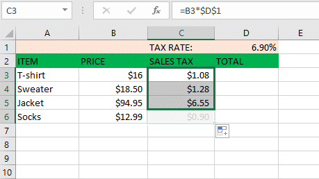
The F4 key in Excel is used to repeat an action. If you’re in a situation where you need to repeat the last action you did in a cell multiple times in other cells, the F4 key can help you do just that but save you quite a lot of time. To activate this key, you press and hold the Fn key in your keyboard, and then you press and release the F4 key (which is located in the first row of the keys in the keyboard). You’re going to need to press and release this combination as many times as you want to repeat that action. Some keyboards don’t feature the Fn key, but no need to worry as the F4 key can work even by itself. The F4, in some instances, is used to decrease the screen brightness, and that’s why the combination Fn+F4 is used.
Freeze Panes
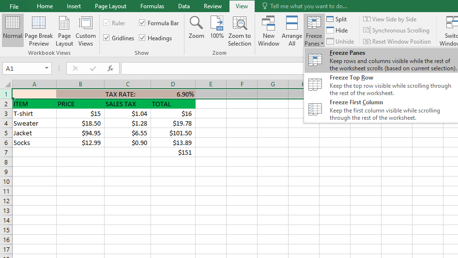
We’ve all been there, had a sheet with hundreds of rows filled with data, and were getting confused when scrolling down. If we have a certain row that can make it easier for us to work, then we can make it visible at all times while scrolling. How do we achieve this? Well, it’s not that hard. You just select the row you want to freeze, and then on the View tab, you click Freeze Panes. By following the same procedure, you can unfreeze the row. This time, you’re going to have to choose the Unfreeze Panes option.
Sum
This function is used to sum up the values of rows and columns in a certain sheet and bring you the results in a heartbeat. Not to underrate the other functions, but this one can easily be one of the most required functions for those working with data.
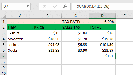
Excel offers many ways through which this function can be used. The first one is the one where you select a cell, and there you type =SUM(, and then you select the cells that you want to add and type) and you press enter and voila it’s done, the result is shown in the cell you previously selected.
However, if you need to sum a large row or column, you can always turn to Excel for help. All you need to do is select the cell you want to be summed up and go over to the AutoSum on the Home tab and finally press enter.
CTRL Z/CTRL Y
When it comes to increasing efficiency, using keyboard shortcuts might be the best option. There are some actions that you don’t need to reach for the mouse at all but instead, press and hold two keys. Two of the most used shortcuts in excel are CTRL+Z and CTRL+Y.
Now, we know we’re not the only ones that we’ve deleted something we shouldn’t have or did something that could jeopardize our task in any way. Well, the first combination, CTRL+Z is just the solution to this problem. This combination is used to undo what was just done, hence saving you and your task.
As for the CTRL+Y, this keyboard shortcut is used to redo the actions we previously undid.
Removing Duplicate
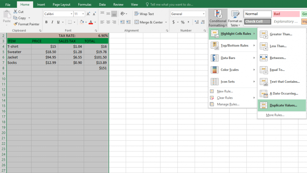
While at times, duplicate data can come in handy, there are times when they just make it more difficult to understand the data. However, one can always remove them and continue the work. If you happen to not be sure where they are situated in your sheet, you first have to locate them. For this reason, you start by selecting the cells you want to check, then you go to the Home tab and choose Conditional Formatting, and then in the Highlight Cells Rules, you choose Duplicate Values. A window opens where you’re going to be picking the formatting you want to apply to the duplicate values and click OK.
Once you locate them in the sheet and decide to remove them for sure, you head over to the Data and choose Remove Duplicate. In the window that opens, you check or uncheck the columns where you want to remove the duplicates.
Flash Fill
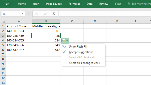
Flash Fill function is there to spare us hours of tedious work and finish it in a matter of seconds. This function is able to identify a pattern based on the data you’re filling and continue the rest of the task for you. You can activate it through the keyboard shortcut Ctrl+E or you can find it in the Data tab. For the Flash Fill to start working, you need to only provide a pattern. So, you insert a new column next to the one with your data. In the first cell of the new column, you type the desired value, and then you press Ctrl+E and enter, and it’s done.
Paste Special
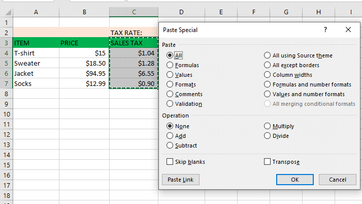
Paste special is this Excel function that gives you more control in how the content looks when pasted from the clipboard. While we’re used to the simple way of copying and pasting by just using the keyboard shortcuts Ctrl+C followed by Ctrl+V, the paste special uses a different keyboard shortcut to paste, Ctrl+Alt+V or Alt+E+S. Initially, you start by selecting the cells you want to copy, press Ctrl+C and then press Ctrl+Alt+V. When these keys are pressed, a dialog window opens where many paste options are provided. You choose the option that you want to.
Add Multiple Row
Even when you have filled enough rows with data, you might realize that you need to insert some more. While you can do so with the right click of the mouse, Excel has thought of an easier and more convenient way and has created a built-in feature that allows you to insert multiple rows. You start by selecting the rows below where you want to appear the rows. You select as many rows as you want to add. Then with the right click of the mouse inside the selected cells, you click Insert and the rows will appear.
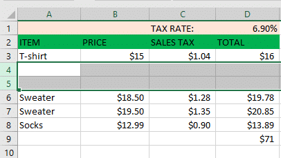
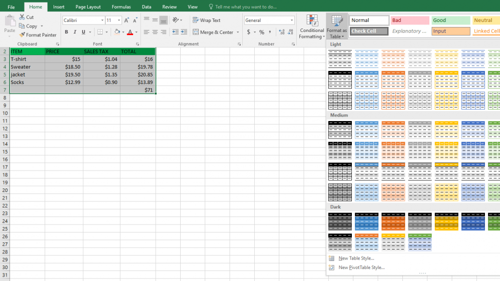
Table Formatting
Excel offers plentiful predefined table styles that you can use to format a table. If you want to format data range into a table, you can select a table style. You start by selecting the cells or a range of cells you want to format as a table. Then, on the Home tab, you click Format as Table, and you choose the table style you want.
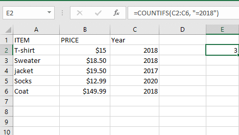
COUNTIFS
The COUNTIFS function is there to count the number of cells in a single range and multiple ranges with a single condition or multiple conditions. Then, it counts only the cells that meet all the criteria specified. The countifs syntax is like this COUNTIFS(range1, “criteria 1”,…).
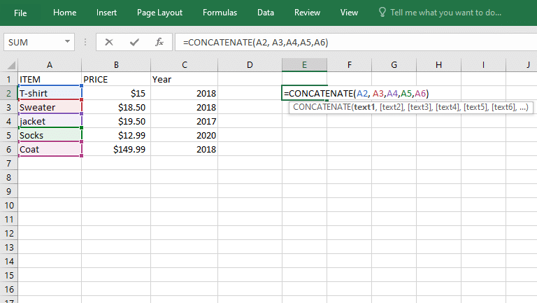
CONCATENATE
The CONCATENATE function is used to join up to 30 text items together and put them in the cell of your choice in the form of the text. The CONCATENATE syntax goes like this =CONCATENATE (text1, text2, text3…).
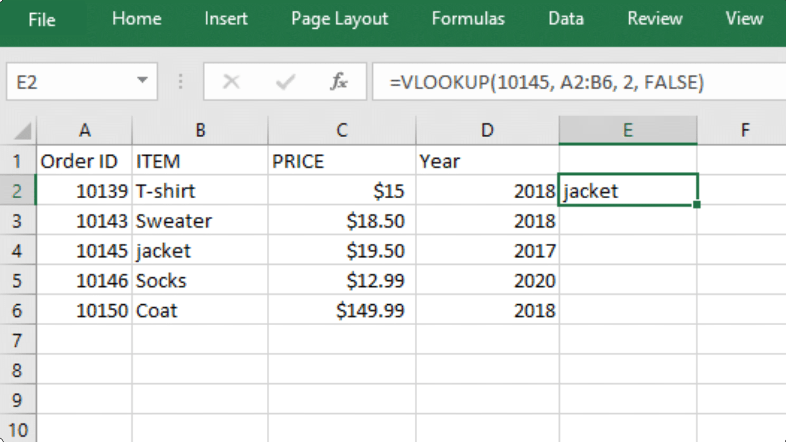
VLOOKUP
The VLOOKUP function is used when one needs to find something in a table full of data. So, how can you use this function., You start by selecting a cell, and there you type =VLOOKUP(). Inside the parentheses, enter the value of the cell that will hold a value followed by a comma and continue to enter the range of cells which you want to be searched, then followed by a comma. For instance, =VLOOKUP(E3,C4:F30,. The final values you add will be the column index number and the lookup value of either TRUE or FALSE. Our finished formula looks like this =VLOOKUP(E3,C4:F30, 5,FALSE).
There you go, guys, all of you who wanted to know about the Excel features for business, we put together 12 of the most used functions and formulas that you as a business major will get to use in the future. All of them are easy to understand and use and can make your job more efficient and increase your productivity level.